One Ring to Rule Them All

Much of this week was shot due to needed car repairs. My timesheet got turned in late, so, no $ next payday... :(

I have to leave early today to pick up Colin, so I'm not sure I have time to accomplish much...

I was planning to look at how/whether I can set delay constraints in Quartus, to see if I can get my ring oscillators to run any faster...

It looks like you have to do it in a Tcl script. There is a command "set_net_delay" which allows you to set a minimum and maximum delay between two nets. I might also be able to use the TimeQuest Timing Analyzer GUI - checking that out now.

Generated a "Net Timing" report for the ring oscillator. The report gives an average Node 1->2 delay of 0.127 ns. Node 2->3 is 0.128 ns. And node 3->1 is 0.117 ns. All together, the total half-cycle period for a ring oscillator transition should be 0.372. So, a full cycle should be 0.744 ns, implying the ring oscillator frequency should be 1.34 GHz! This is more than twice the frequency (~550 MHz) that I actually observed, so something is fishy.

OK, I'm looking now at the ring oscillator layout in Chip Planner, and it appears that all 3 of the inverters have been synthesized in a couple of cells that are located right next to each other. So, Quartus is already doing as best it can to minimize the ring oscillator delay. The only question is, why does the actual ring oscillator frequency turn out to be only about half as large as expected? Perhaps I need to double-check my measurement setup with the carry-save counter, or try to figure out if I can do a more direct measurement of the ring oscillator output, perhaps through the CLK_OUT coax connector. Let's try that early next week.

Testing the new RO

Ray wanted to test the comparators today, but we decided that since we expect them to work anyway, we might as well hold off on that until needed to help diagnose any problems we might run into with the actual TDC readout. But figuring out the TDC output will take a more focused effort by Mike over several weeks. Mike will start on that after the end of the semester (i.e., after this week, since it is still finals week).

In the meantime, I am continuing to work on testing our own ring oscillators on the DE3 board. To count (half-) cycles, I wrote a 64-bit dual-edge-triggered carry-save counter in structural VHDL, using the recursive dual-edge triggered register I wrote earlier. I'm not sure if the counter will be able to keep up with the ring oscillator (quite possibly not), but if not, I can back off to a larger size of ring oscillator (e.g., 5 stages instead of 3), and still do a little better (in terms of time resolution) than I could with a single-edge-triggered counter. Anyway, we will see.

Created a simple schematic module test_ro.bdf that just uses the ring oscillator to drive the clock of the 64-bit counter. Having some problem now compiling my recursively generated register (pde_reg.vhd)... Aha, it was just some confusion between parent/child signal names in the recursive port map. Fixed it by passing the I/O through internal signals with different names.

I'm looking at bit 30 of the counter on the scope; this should have a period that is 2^30 (about a billion) times longer than the ring oscillator period. (Because I am using the dual-edge triggered flip-flops, bit 0 of the counter should have the same period as the ring oscillator, and bit N has 2^N times longer period.) Unfortunately, I am seeing nothing on this signal (no change; constant 0). Trying ring oscillator length 5 stages: Still no dice. Now trying 7 stages: That works. Hm, I think this means I have to revert back to single-edge-triggered flip-flops - the dual-edge triggered ones aren't buying us anything.

OK, with the single-edge-triggered flip-flop, and a 3-stage ring oscillator, bit 20's period is 3.75 ms. Thus, bit 0's period is 3.58 ns. Thus, the actual clock period is 1/2 this, or 1.79 ns. Thus, the ring oscillator frequency is 559 MHz. No better than I saw on the DE2! Maybe I should try imposing some time constraints, or something... Anyway, do that tomorrow...

Crossing the Threshold

I think today Ray wants us to test the threshold levels produced by the DACs. While I'm waiting for him to get here, I'll keep working on my own TDC code.

After some thought, I think that the pseudo-dual-edge-triggered flip-flops are probably not going to be able to keep up with the (3-inverter) ring oscillators, because of the number of LUTs worth of delay (2 perhaps) in the interface logic (two levels of XOR gates) that turns the two single-edge triggered registers into a dual-edge triggered one. However, I am not 100% sure, especially since the half-adders and the XORs may get compiled together into a single LUT, so I am going to try it anyway. Also, even if we go to a 5-inverter ring oscillator, if we cut that period in half using the PDEDFF, that will be 2.5 inverter delays between active edges, which is still better than 3.

Found RTL_ATTRIBUTES.VHD online, added it to project. I think it is from IEEE Std 1076.6TM-2004, IEEE Standard for VHDL Register-Transfer Level (RTL) Synthesis. However, it doesn't appear that Quartus supports all of these attributes yet.

OK, we verified the ability to set the DAC output levels for the comparator thresholds through the LabView interface. Here is the mapping from LabView VI elements to net names in the PCB schematics/layout and reference designators of the test points:

Designation in vth_test1.vi Header PCB net
--------------------------------- --------- ----------

1. VTH (High) (Low Energy) 2 J37 VTH5
2. VTH (Low) (High Energy) J38 VTH6
3. VTH LOW HS 2 J33 VTH1
4. VTH HIGH HS 2 J34 VTH2
5. VTH 5 J35 VTH3
6. VTH 6 J36 VTH4

Also, we started looking at how to probe the LVDS comparator outputs. Here is an example. We should probably rename the nets in the PCB layout to be more descriptive.

PCB nets Quartus net Pkg. pin Net (PCB) Hdr.
------------- --------------- ----------- ------------ ------

1. PMT_1,VTH1 P1VTH[1] PIN_F17 N9384431 J53
2. ...

Back on the Quartus design now. I have test-compiled the PDE_DFF, PDE_REG, and RING_OSC modules, and am ready to put them into a test circuit in my DE3_GPSAPP project. Oh, first I need to bring in my carry-save counter and integrate it with the PDE_REG. However, I have to go now, so that will have to wait till next week.

Virtual Machining

Parking was tight today, probably a lot of students have finals/final projects. Had to park over at Engineering and take the bus. I will also have to leave early today (about 4pm). I will be glad when it's

Thinking today of starting on the new ring oscillator characterization stuff, including trying dual-edge triggered registers for higher resolution. Looked in Ashenden (Designer's Guide to VHDL, 3rd ed.), and it looks like we want a recursive generate architecture.

Also, today Ray wants to compare VirtualBox vs XP behavior of the existing LabView interface. Oops, I messed up the VM by trying to run it again simultaneously from another account! Now we are having to try to restore the files from the virtual HD.

It's Moanday... Ugh.

Today started with being woken up WAY too early by the stupid cat, followed by not being able to get back to sleep, and feeling rather unwell for the next several hours. Finally was able to get myself together & out the door. Then followed a >$500 car repair payment (following an extended wait in line at the overworked mechanic's shop to pay for it & pick up my car). Finally, on the way to work from the shop my car started overheating, and so I had to stop & check the oil (which was not low), and then I had to turn off the A/C for the rest of the trip (which seemed to work around the problem, for now). Stereotypical Monday!

When I got in, I checked out the status of the XP machine, which Ray said was still stuck on update 26, which is where I think it was when I left on Friday. Apparently IE8 had a dialog open and was insisting on getting a definite answer to a stupid "want to participate in sending extra data to Microsoft" question before it finished installing itself. Got past that and the remainder of the 90-something updates are now installing. Hey Microsoft, how about making your software engineers use sound coding practices, so they don't create so many holes in the first place? Then maybe you wouldn't need quite as many "critical security updates."

As you can tell, I am in a rather foul mood today. Not unusual for the day after the kids go home, I suppose. On these days particularly, I despise my sociopathic ex-wife for manipulating me into marrying her, and then taking my only child away. It seems worse than usual today though. I suppose it's the stupid cat's fault - I'm grumpy because I didn't get enough sleep. After waking me up early for no reason, she jumped up onto my (bare) shoulders while I was at my desk checking my email, and I really wasn't in the mood for it, so I just shoved her off of me and let her fall to the floor - since I was already tired & grouchy and I REALLY didn't want to deal with her probably raking her claws into my unprotected skin, which is what usually happens when she is trying to get down safely from her perch on my shoulders. Maybe she'll think twice before the next time she jumps up there.

Anyway... When I left Monday, I was about to try running the DRAM demo under the Nios II IDE debugger. OK, it is running now (getting past where it was stuck on Friday), but the memory test failed!! Each time I tried it! First time at i=0, subsequent times at i=47.... Let's try rerunning it in RUN mode instead of DEBUG mode... Now it fails at i=94... Then i=47... repeatedly. OK, one more thing to try: Recompile in Quartus to pull latest compiled firmware into the FPGA bitstream, then monitor the output from nios2-terminal. Again, the test fails, this time with i=47 first, and then i=0 each time (but with different read vs. expected values).

Ah, OK, RTFM! When I started the demo by running the Demo Batch file (in "C:\LOCAL\DE3_demonstrations\150\DE3_DDR2\demo batch\de3_ddr2.bat"), instead of manually, it worked. I guess that means I need to figure out what's different about the way the demo is being run from within the batch file... Hm... Looking at it, there seems to be nothing unusual. Let's dissect it piece by piece:

First line:

%QUARTUS_ROOTDIR%\\bin\\quartus_pgm.exe -z -m JTAG -c USB-Blaster[USB-0] -o "p;DE3_DDR2_Q8.sof"

Running quartus_pgm.exe with the --help=z, etc. flag says:

"-z | --haltcc: Halts the on-chip auto-configuration controller of the device to allow programming via the JTAG interface."

"-m ... specify which programming mode to use."

"-c ..." (obviously)

"-o ..." and "p;" means "Program"

Nothing unexpected there. Then, the .BAT file just sets up some path variables and runs Cygwin bash on the de3_dd2_bashrc script. That just runs the standard "nios_bash" script for sopc_builder (which I think the normal nios shell must do also, right?), sets up some aliases, then does:

nios2-download ddr2_TEST.elf -c USB-Blaster[USB-0] -r -g
nios2-terminal -c USB-Blaster[USB-0]

The --help for nios2-download says: -c specifies the cable (clearly), -r says to reset the target SOPC system before use, and -g says run processor from entry point after downloading. Meanwhile, the -c argument to nios2-terminal just sets the cable.

Who knows, maybe if I run it the usual way, it doesn't start from the right entry point, or something... I guess it doesn't matter because in a pinch I can always load/run my design using the command-line tools instead of the GUI, and just imitate what the batch file is doing...

Still, it would be nice to be able to use the interactive debugger... Right now it gives some kind of warning about a version mismatch... Forcing a recompile (i.e., like make clean; make) of all the firmware, to see if that helps... Nope. Now trying: Regenerate the SOPC system in SOPC Builder, recompile Quartus design, and recompile firmware... Argh, still same problem.

DRAM'ed if you do, DRAM'ed if you don't

I'm getting ready to expand my project to be able to use the 1 GB DDR2 667 MHz SDRAM (SO-DIMM card) that came with the DE3 board. ("DDR2 SDRAM" just means the 2nd version of the standards specification for interfacing to double data rate synchronous dynamic random access memory.)

First, looking at instructions in the DE3 user manual. It says that due to a limitation of SOPC Builder, only 256MB of the DRAM can be accessed if SOPC Builder is used. The demo is limited to 256 MB. So, if I want to use the full 1 GB DRAM, I might have to first learn how to build the project without SOPC Builder (using command-line tools, I assume). However, it might make more sense to first just limit the size of my memory buffer to 256 MB. That will take about 27 seconds to fill at 10 Msps, at 1B/sample. Actually, it might be wise to time the OCXO's falling edges as well; so then that's 20 Msps, and the memory will fill up in about 13 seconds (assuming we can write it that fast).

First, I'm copying the entire DE3_Demonstrations\150 folder from C:\Users\Public\Documents\AlteraDE3boardCD to C:\LOCAL\, so that I can access it a little more conveniently.

Opening the DE3_DDR2_Q8.qpf Quartus project in Quartus 9.1. (Sometime I should perhaps upgrade to Quartus 10, but for now - if it ain't broke, don't fix it. :) Looking at the SOPC Builder design. It looks like it uses a couple of PIOs to communicate with the DDR2 controller. There is also an "altmemddr" device. That dialog is pretty complicated! There are also some Tcl scripts you have to run to set up the controller IP, the source code of which is not viewable.

Also viewing the Nios 2 code. Looks like I modified it slightly earlier (just to print a message, to make sure I could modify it).

Recompiling the Quartus project now, just to make sure I can (in the new location).

OK, my modified software is loaded and running. However, the memory test seems to be taking a while... Several minutes just to test 256MB? It's running at half speed, but that doesn't fully explain it... Oh, maybe it is the slow clock speed of the Nios 2 that's the problem...

Meanwhile, regenerating the SOPC system, to make sure I can do that... Yes.

The run still seems to be stuck, recompiling the software now, to test that and so I can run in debugger...

Time to go to Gainesville, but we will continue this next Monday...

The Timekeeper Speaketh

(LOL, I'm imagining I'm a Marvel-style Cosmic Abstract called "The Timekeeper," whose job it is to measure time on all scales, from Planck scale to cosmic.)

My thinking as to next steps, at the moment is this:

1) Put the ring oscillator and carry-save counter on the DE3 board, measure ring oscillator frequency. Expecting around a GHz.

2) Try using the dual edge-triggered flip-flop to double the frequency again.

3) Reconstruct our input-capture circuit at this faster timescale, for registering 10MHz OCXO edges against the ring oscillator cycle counter. (We don't want to use the 50MHz on-board clock since it is less stable.) At 2 GHz, we could count ring oscillator cycles for >292 years without rolling over a 64-bit counter (although, since the cycle counts will always be in the general neighborhood of 200, give or take 100, there would also be no information lost by just using a 8-bit counter, and calculating the deltas by just subtracting modulo 256). If there are any metastability problems due to the short cycle time, fix them by adding some latch stages.

3) Learn how to use the DRAM in the DE3 SIMM card slot, and use it to store 1 GB of time delta data. Using 8-bit data values (adequate to cover a pretty range of deltas, from say 72 to 327), this gives us 1 billion (well, 2^30) samples. At the 10MHz OCXO frequency, that gigabyte of data will take only 100 seconds to collect. However, transferring it to the server over 56Kbaud serial would take about 2 days. Instead of doing that, I should either (a) collect less data, or (b) copy it to a file on an SD card, which I can then transfer to the server physically.

4) Do the Allan deviation computation for this dataset in C (instead of Scilab, which is too slow). In C, each pass through the GB of data (once it's loaded into RAM) should only take a few seconds, at most. Generating a thousand data points for a high-res data plot would then take around an hour, which is quite tolerable. Again, however, the range of timescales covered by the plot will only be up to 100 seconds. The minimum of the Allan deviation curve may well be below that point, though. (If not, we can set up the Ethernet on the DE3 board, and collect more data by streaming it at 10 MB/s to the server in real time while the data collection is running.)

5) Find the minimum of the Allan deviation curve for the ring oscillator vs. the OCXO. This will tell us the optimum window size T (hopefully <100 sec.) for measuring the ring oscillator frequency most precisely.

6) Implement a circular storage buffer of that size (10 MB/s)*T, and use it to store the last T amount of time worth of deltas, and also keep around a register large enough to store the running sum of all the deltas currently in the window. Add in the new values, and subtract out the old ones. This then becomes a proportional representation of the average frequency of the ring oscillator (relative to the OCXO) over the last T amount of time.

7) This technology then, I think, becomes sufficient to measure sensor event times with resolution about equal to the half-period of the ring oscillator (about 0.5 ns). We can measure threshold-crossing times by using an HSMC daughter card to do DAC conversion, to generate the threshold levels to send into the FPGA's LVDS input comparators. Then, when a pulse comes in from the PMT (or APD), we can capture that input transition, and store the threshold-crossing time, measured in ring-oscillator half-cycles since the last OCXO clock edge, as well as OCXO cycles since the start of the run. The data sent to the server can include the sum of the ring-oscillator cycle-count deltas from the most recent size-T window, which tells the server (quite accurately) the present mean frequency of the ring oscillator. Furthermore, we could even keep a running tally of the 1-cycle Allan variance over this window, which would give us an up-to-the-minute measure of the time deviation inherent in extrapolating times using the ring oscillator over the 100 ns OCXO cycle. (We could refer, instead, to OCXO half-cycles, but the problem with that is that the duty cycle of the OCXO is only specified to +/-5%, so we would have to first characterize the variability of that quantity as well.)

I think that's as far as I'm going to look ahead as to my plans for this line of development, for now. Let me get some feedback from Ray on this first.

He says he'd like to proceed with Sachin's board anyway, for now at least, but I might still spend a little time tinkering with the DE3.

On tap for Monday: Open Science Grid meeting, and installing LabView on the XP partition of the Acer (now that Juan has restored access to the Windows 7 partition and we know the state of that machine is stable). Right now, I am installing critical Windows Updates, to get the machine ready for the LabView install.

Running Rings around the Oscillators

Working from home today because my car battery is dead. :(

Today, SUCCESS at building a fast ring oscillator on the DE2 board (in VHDL). The speed of course depends on a lot of things (placement, routing, temperature), and so differs quite a bit between runs, but the fastest speed I have seen so far is 666 MHz.

I measured the frequency by building a fast counter with a carry-save architecture, which can keep up with the ring oscillator. Bit 6 of the counter goes 128x slower than the underlying clock and was measured at up to ~5.2 MHz using my cheapo home oscilloscope (which in theory can measure signals up to 25 MHz but which in practice has trouble getting above 10 or so, due I think to crappy probes.)

To get this working, I had to learn how to set the KEEP attribute in VHDL, to keep it from compiling away my ring oscillators and clock fanout buffers.

The Stratix II should be able to go even faster, I'm guessing pretty close to 1 GHz at least.

If I use dual-edge-triggered flip-flops in my counter (I should try that soon), we could count half-cycles, and so effectively measure time at 2 GHz (every 0.5 nanosecond).

So what I'm thinking now is that we could just directly sample the comparator outputs at the frequency of one ring oscillator to get nanosecond time resolution, without even having to worry about fine-tuning two different ring oscillators to be close together in frequency, and then counting cycles until the phase crossover to get sub-cycle resolution, like Sachin has been trying to do. This seems like it would be a lot easier and more straightforward.

The ring oscillator frequency can be easily calibrated against the time sync signal by simply latching the counter value when the time sync goes high, just like how we are registering the OCXO against the GPS PPS signal now.

So basically, what I'm thinking now is, we should completely redo Sachin's Quartus design with a totally different architecture. Maybe even just use the serial port for communication, like we were planning to do originally (and then we can use Wi-Fi instead of Wireless USB, and get better range). However, this might mean we have to redo all the LabView interface stuff (assuming we still want to use LabView).

If we can, also get a Nios II core on there, so that we can manage the I/O and high-level functionality in C, instead of having to do custom gelware for that part.

We do still need to interface with the DACs to set the comparator thresholds, but that shouldn't be too difficult.

Here's a video of today's test:

Weekend Thoughts

I started thinking about the project today, and had an idea.

Presently one of the major sources of error we are dealing with in our time measurements is the quantization error due to the fact that we are only sampling the PPS signal from the GPS at 100ns intervals. The standard deviation of the resulting phase error is 100/sqrt(12) = 28.9 ns.

Meanwhile, the GPS module itself uses a 16.368 MHz clock, which means the phase noise due to the quantization error in that clock is less, probably 61.1/sqrt(12) = 17.6 ns.

We could reduce our contribution to the phase error in half if we use dual-edge flip-flops to sample the signal every 50 ns; then the RMS phase error will only be 50/sqrt(12) = 14.4 ns.

However, we could do better yet if we implement our own TDC directly on our FPGA board. Spent some time today trying to do this with the DE2 board I have at home...

Now what?

What to work on today?

* Emailed Brian Stearns @ DeLorme to let him know that the Allan deviation problem is resolved.

* Maybe I should update my "Recent Results" page with the new graphs... OK, did that.

* Updated my latest graph to clean up the colors and titles & add back in some of the curves that accidentally got deleted earlier:

Untitled Blog Post

I couldn't think of a clever title today. My brain is kinda fried from being busy lately. Anyway, what to do today?

* Ray called me at home this morning to ask about Xmath status. Checked status of Xmath requisition when I got in. It is indeed marked as "PO dispatched". Should we ask Purchasing to email us a PDF so we can get it to LeCroy more quickly? Also, should we check Sonya's office to see if the license arrived in a physical package? Ray says he will call LeCroy.

* Guess I should spend most of today continuing to work on material for the journal article.

* I was thinking on the way to work about whether/how we could obtain more accurate GPS times by averaging the relative OCXO/GPS frequency over longer periods than one second and interpolating a best-fit time trajectory. According to the OCXO datasheet, the 1-sec. Allan deviation of the OCXO is nominally 5e-11. So, we'd expect the OCXO's absolute time deviation over n seconds to be 5e-11*sqrt(n/3), I think... So, suppose we averaged the trajectories over a 10,000-second (2.78 hour) period. That gives a time deviation for the OCXO of 2.89 ns. Meanwhile, the Allan deviation for the OCXO vs. GPS for frequencies averaged over that period is (from our 10-day dataset) 2.20e-9. So together, I think this means we should have no worse than about 2.9 ns inaccuracy for absolute times inferred by averaging over that window size.

We can maybe do a little bit better than this if we optimize the window size further. The below graph plots the raw (red) and quantization-error-corrected (blue) values of the Allan deviation, and the expected time deviation due to inherent OCXO instability, as a function of the size of the averaging window. The max of the blue and yellow curves is minimized at a window size of about 6,918 secs. (1.92 hrs.), at which the adjusted relative Allan deviation is 2.41e-9, and the expected OCXO time deviation is 2.40e-9 secs.

So, what is this saying exactly?

First, the corrected Allan deviation says that, supposing that we measured the OCXO vs. GPS average relative frequency over a ~2 hr. period, we would expect the frequency so measured, even in the absence of any quantization error, to be offset from the actual mean relative frequency over the period consisting of the current 2 hr. period adjoined with the following 2 hr. period by an amount that is distributed with a standard deviation of +/- 2.41e-9, expressed as a multiple of the actual relative frequency. Given a nominal OCXO frequency of 10 MHz, this means that the expected frequency deviation of the OCXO vs. GPS is about 0.0241 Hz. But, the OCXO is really much more stable than that. So the measured relative frequency deviation is actually due almost entirely to variations in the frequency of the PPS signal from the GPS. The GPS PPS signal is supposed to be at 1 Hz, so this means that its average frequency over this size time period is offset from what it ought to be by a standard deviation of 2.41e-9 nHz. Translating frequency deviation to time deviation, this means that (if it were free-running) the GPS's unit's idea of the total time elapsed since the start of this ~2hr period could be off by as much as ~29 microseconds (std. dev.)! This makes sense, particularly with respect to the ~50us size of the phase excursions that we (not infrequently) do see, due to time-lock being lost as a result of the limited sky visibility through our window. However, except at times when time-lock is actually lost and a major (typically many-microsecond) phase excursion is happening, the GPS unit's clock is not really free-running, but is phase-locked with the actual GPS signal from the satellites. So, during such "good" periods, we can expect the actual time deviation of individual PPS pulses could be much less than the 116 nanosecond value. Typically, TRAIM reports that it is; although at present we are not yet confident in these reports. (Since they seem inconsistent with the Allan deviation values we're seeing, which indicate a larger time uncertainty.)

Let's think a little more carefully about how to model all this. First, there is "real" (UTC/USNO) time, flowing (more or less) equably, which the GPS satellites know, and which our GPS module keeps in sync with, albeit imprecisely. The GPS unit includes an internal clock which experiences random frequency fluctuations on short timescales. Our Allan deviation measurements are evidence of this.

However, it occurs to me that I don't really know if our Allan deviation measurements would still be accurate during intervals where time lock isn't lost. I need to redo the Allan deviation calculation for a known "good" interval. The first 40,000 or so seconds of our 10-day run looks pretty good; I should probably redo the Allan deviation calculation just for that portion. Working on that now.

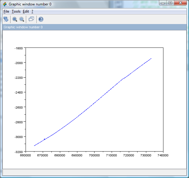
Actually, let's take the 68,000-sec. (~18.9-hr.) interval from 665,000 to 733,000 seconds into the run, which is pretty smooth:

Indeed, when we plot the Allan deviation just for this interval, we find it is much smaller than the overall plot for the entire run:

In fact, at least for small window sizes, this deviation (blue line) seems to be dominated by the quantization error:
The yellow line shows the quantization error's contribution to the total Allan deviation, and the green line shows the adjusted version of the blue line if the variance for the quantization error is subtracted from the total Allan variance.

Let's throw in another curve, this one from the first 40k seconds:

That looks pretty similar to the one from the other "flat" period.

But all this, now, totally throws into question a bunch of my recent conclusions, including the notion that the Allan deviation ought to scale down with 1/sqrt(t) - although it may still do so in some regions of these curves - as well as the impression that the GPS unit's clock had an inherent frequency instability on the order of 1.67e-7 (1-sec). Instead, in the new curves it is as low as 3.14e-8 (@1 sec), or 31.4 ppb. This makes more sense, from the perspective that the GPS clock's phase is being adjusted using the satellites. In fact, it is in line with the typical ~30ns accuracies that we get from the TRAIM algorithm. Actually, just did a measurement of the average nonzero TRAIM accuracy over the 10-day run, and it was 18.1 ns. From quantization error alone, the standard deviation of time error would be 28.9 ns. And the DeLorme doc specifies 62 ns. However, using the 1/sqrt(12) rule gives 17.6 ns, which is pretty close to what TRAIM reports. Actually I should calculate the RMS TRAIM accuracy, OK, that is 21.1 ns, also still close. Probably, however, I should make a worst-case assumption and put it back up at around 60 ns, which is about the documented accuracy from DeLorme as well as the "corrected" accuracy from the 48ks run segment.

Now, this is nice: If we average over 151-s intervals, and use the purple line from the 1st 40ks, we can get theoretically an accuracy of 372 ps. Really meaning, the frequency deviations at that timescale are only 3.72e-10, so if take a frequency measurement based on the last 151s, it should be only 372 ppt from the "real" mean frequency for that timescale... And meanwhile, extrapolating OCXO times over that timescale should only result in time errors of that magnitude. So combining these we might be able to get absolute time accuracy less than a nanosecond! Need to think some more about this... Here's the intersect graph...

A Modest Proposal

* Texted Ray over the weekend about the possibility of designing a scintillator-based Geiger counter substitute that used the iPhone as a user interface. We talked about it on the phone for a little while this morning.

* Ray asked me to write up a paragraph or so of text for the proposal based on the recent results on the GPS timing system. Here's what I've got so far, about a page. Asked Ray for some feedback on what I should cut.

We recently completed a series of tests of the DeLorme GPS2058 module which we are using in our demonstration system for purposes of assigning absolute time stamps to individual shower detection events. We characterized the time stability of the module by comparing its output against a high-precision 10.0000 MHz OCXO (oven-controlled crystal oscillator) having 10 ppb (parts per billion) frequency stability, used as a frequency reference, and plotted the relative Allan deviation (a measure of frequency instability) between these two timing sources (below left). After correcting for the expected quantization error (due to the 10 Msps sampling rate) of ±50 ns, we found that the fine-grained Allan deviation (between adjacent 1-second frequency averaging windows) was 1.67 × 10⁻⁷ (in dimensionless units), which, at the 10 MHz OCXO frequency, translates into ±1.67 Hz of relative frequency instability, or in other words, ±167 ns RMS deviation from the mean in the time of arrival of individual PPS (pulse per second) timing pulses received from the GPS module. This then implies a comparable lower bound to the uncertainty of absolute time measurements based directly on the GPS PPS edges. We could improve the accuracy somewhat by averaging the GPS time readings over longer intervals, but (given the 10 MHz OCXO frequency) not to better than a ±25 ns lower bound that would be set by quantization error even if we used dual-edge triggered flip-flops in our input capture circuit to achieve 20 Msps. But without using differential GPS or military-grade access codes for improved accuracy, the GPS network does not offer users any better time resolution than around that level in any case.

If we assume, for the time being, an uncertainty of ∆t = ±160 ns for the absolute time measurements at a given detector site, then this limits the angular resolution for determinations of the bearing of a large-scale (atmospheric or interstellar) cosmic-ray shower detected at multiple sites. For two detectors separated by a straight baseline of length b < 7,926 km (diameter of Earth), and for an interstellar shower coming from a heading on the celestial sphere at an angle θ away from the baseline axis, the uncertainty in the measurement of θ is given by |∆θ| = c∆t/b (sin θ)⁻¹, in the approximation where
c∆t << b, and where the time reference at the other detector is assumed to be perfectly accurate. The same formula also applies to atmospheric showers for baselines that are less than that of a typical shower diameter at ground level (a few km). In the figure at above right, we plot this quantity for a variety of baseline lengths and source elevations (relative to the baseline axis). So for example, for two sites that are spaced 1,000 km apart, the angle θ for an interstellar shower coming from a direction nearly orthogonal to the baseline axis could be determined to within about 10 seconds of arc once the coincidence between the two detection events (occurring ~1 ms apart, or less) has been identified.

OK, now done a shorter (1 paragraph) description:

Our demonstration system for timestamping cosmic-ray shower events utilizes a DeLorme GPS2058 module for (once per second) absolute time synchronization, together with a Connor-Winfield 10.0000 MHz OCXO (oven-controlled crystal oscillator) with 10 ppb frequency stability for more fine-grained, higher-precision time measurements. We recently completed a series of tests on these components for purposes of verifying the absolute accuracy that we can expect to obtain for comparison of event times between detector sites; our empirical results and analysis will be described in detail in an IEEE journal article (currently in preparation). Our measurements of relative Allan deviation (frequency instability) are shown in the figure at left below. From this data, we inferred that there is an estimated ±167 ns RMS jitter in the time of arrival of individual timing pulses from the GPS unit, which is likely traceable to the low-offset phase noise of the TCXO (temperature-compensated crystal oscillator) which is used for timing purposes inside the GPS module. Given the implied time uncertainty of |∆t| ≈ 160 ns, we can calculate the uncertainty |∆θ| = c|∆t|/b (sin θ)⁻¹ in the inferred angle θ between a shower's heading and the baseline axis between two detector sites that are a distance b apart (below, right). So for example, given two detector sites spaced 1,000 km apart, the off-axis angle θ for an (interstellar) shower coming from a direction nearly orthogonal to the baseline axis could be determined to within about 10 seconds of arc, once the coincidence between the two detection events has been identified.

Also digging up some other graphs to post on project page... OK, all of the recent graphs (and some explanation discussion) are now posted at http://www.neutralino.org/projects/cosmici#TOC-Recent-Results.

Quantization Error Redux

Ray says that Sachin & Vaibhav are out of pocket for a little while. We'll wait and work on the board ourselves when we have time. In the meantime, I am reading a book on USB at home in the evenings, which will help us out if we need to debug or make changes in the communication.

My plan for today is to work on the new analysis of how the quantization error affects the Allan deviation by developing a program to do the calculations numerically.

I decided I wanted to first try just writing the new analysis in C/C++ (for faster development since I am most familiar with this language). I liked the NetBeans IDE that Gordon introduced me to, so I will try using it. I already reinstalled it with C/C++ support added a few weeks ago. Today, registered my installation with Oracle. Realized it needed Cygwin for the underlying gcc compiler. There is already a Cygwin environment in the Nios II IDE, but I decided instead of trying to use that one with NetBeans also, it would be cleaner to just install another one for general use. Did that, selecting gcc/make/standard libraries/gdb to install. Also included USB development support in case we need to do any raw USB coding in C. Created a new project "AnalyzeQuantErr"; now ready to start programming...

OK, I got to the core of my calculation, which is the following integral (expressed in Mathematica syntax):

Integrate[PDF[NormalDistribution[mu, sig], Phi2 - Phi1]*
PDF[NormalDistribution[mu, sig], Phi3 - Phi2], {Phi1, -(1/2), 1/2},
{Phi2, x2 - 1/2, x2 + 1/2}, {Phi3, x3 - 1/2, x3 + 1/2}]

Unfortunately, Mathematica is unable to integrate the result over Phi2, although it does manage to do the other two integrals. I tried all possible orders of integration, and did not achieve any better result. So, it looks as if I will have to numerically evaluate the following integral over Phi2:

Integrate[(1/4)*(Erf[(-(1/2) + mu - Phi2)/(Sqrt[2]*sig)] -
Erf[(1/2 + mu - Phi2)/(Sqrt[2]*sig)])*
(Erf[(-1 + 2*mu + 2*Phi2 - 2*x3)/(2*Sqrt[2]*sig)] -
Erf[(1 + 2*mu + 2*Phi2 - 2*x3)/(2*Sqrt[2]*sig)]),
{Phi2, -(1/2) + x2, 1/2 + x2}]

Fortunately, the error function erf() is included in the C math library already, so I don't have to write code to evaluate that as well.

OK, the program is done now, and I ran it and it produced sensible-looking results:

Here's the same graph on a log-log scale, which emphasizes the low end of the scale more:

As we can see, when the inherent frequency variation of the oscillator over the 1-second window size approaches 0, the measured Allan deviation due to quantization error approaches 1/2 cycle. This probably makes some kind of sense, since quantized phase measurements can be off by at most (+/-) 1/2 cycle, and 1/2 is also the RMS error of the quantized deviation that I obtained before by integrating the Dirac delta function under the assumption that the quantization errors of the 3 points x1,x2,x3 are independent & uniformly distributed in the range [-1/2,+1/2] cycle.

And, when the inherent frequency variation of the oscillator (for frequencies averaged over 1-second intervarls) increases well above +/- 1 cycle per second (standard deviation), the Allan deviation asymptotically approaches the actual standard deviation, which is correct since the quantization error then becomes relatively insignificant, and Allan deviation is designed to give the actual deviation in the case of a white noise model of the oscillator frequency fluctuations.

So, this seems like a good, solid theoretical result.

Meanwhile, let's apply this to our data set. We measured a 1-s Allan deviation of 1.7407 cycles. Going backwards through the above curve, we find that the actual standard deviation of frequency is 1.6674. Lo and behold, this is exactly the same as we had computed before by just using a simple quadrature combination of quantization error and inherent frequency variation, using the standard deviation of quantization error of 1/2 cycle that we had already obtained by our simpler analysis (integrating Dirac delta function)! This suggests that the above curve, arrived at by a complicated numerical integration procedure, could have been reproduced using the simple quadrature rule. Indeed, the curve obtained that way is indistinguishable to within 1/1000 cycle, which can be easily accounted for by the imprecision inherent to numerical integration.

This is all a good sanity check of the analysis - the two methods I used (simple quadrature rule & more detailed model) obtain the exact same result. So, I am now confident in this method (either/both method) for accounting for the quantization errors. Of course, it all assumes Gaussian white noise.